What is the institutional detail that makes electricity special? Its in the physics that I will summarize with a model of DC current in a resistive network. Note that other sources, like Wikipedia give other reasons, for why electricity is special:

Electricity is by its nature difficult to store and has to be available on demand. Consequently, unlike other products, it is not possible, under normal operating conditions, to keep it in stock, ration it or have customers queue for it. Furthermore, demand and supply vary continuously. There is therefore a physical requirement for a controlling agency, the transmission system operator, to coordinate the dispatch of generating units to meet the expected demand of the system across the transmission grid.

I’m skeptical. To see why, replace electricity by air travel.

Let {V} be the set of vertices and {E^*} the set of edges a the network. It will be convenient in what follows to assign (arbitrarily) an orientation to each edge in {E^*}. Let {E} be the set of directed arcs that result. Hence, {(i,j) \in E} mens that the edge {(i,j)} is directed from {i} to {j}. Notice, if {(i,j) \in E}, then {(i,j) \not \in E}.

Associated with each {(i,j) \in E} is a number {x_{ij}} that we interpret as a flow of electricity. If {x_{ij} > 0} we interpret this to be a flow from {i} to {j}. If {x_{ij} < 0} we interpret this as a flow from {j} to {i}.

  1. Let {\rho_{ij}} is the resistance on link {(i,j)}.
  2. {c_i} unit cost of injecting current into node {i}.
  3. {v_i} marginal value of current consumed at node {i}.
  4. {d_i} amount of current consumed at node {i}.
  5. {s_i} amount of current injected at node {i}.
  6. {K_{ij}} capacity of link {(i,j)}.

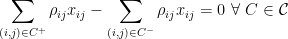
Current must satisfy two conditions. The first is conservation of flow at each node:

\displaystyle s_i + \sum_{k: (k,i) \in E}x_{ji} = \sum_{j: (i,j) \in E}x_{ij} + d_i\,\, \forall i \in V

The second is Ohm’s law. There exist node potentials {\{\phi_i\}_{i \in V}} such that

\displaystyle \rho_{ij}x_{ij} = \phi_i - \phi_j\,\, \forall (i,j) \in E.

Using this systems equations one can derive the school boy rules for computing the resistance of a network (add them in series, add the reciprocals in parallel). At the end of this post is a digression that shows how to formulate the problem of finding a flow that satisfies Ohm’s law as an optimization problem. Its not relevant for the economics, but charming nonetheless.

At each node {i \in V} there is a power supplier with constant marginal cost of production of {c_i} upto {S_i} units. At each {i \in V} there is a consumer with constant marginal value of {v_i} upto {D_i} units. A natural optimization problem to consider is

\displaystyle \max \sum_{i \in V}[v_id_i - c_is_i]

subject to

\displaystyle \sum_{j: (i,j) \in E}x_{ij} -\sum_{j: (j,i) \in E}x_{ji} - s_i + d_i= 0\,\, \forall i \in V

\displaystyle \rho_{ij}x_{ij} = \mu_i - \mu_j\,\, \forall (i,j) \in E

\displaystyle -K_{ij} \leq x_{ij} \leq K_{ij}\,\, \forall (i,j) \in E

\displaystyle 0 \leq s_i \leq S_i\,\, \forall i \in V

\displaystyle 0 \leq d_i \leq D_i\,\, \forall i \in V

This is the problem of finding a flow that maximizes surplus.

Let {{\cal C}} be the set of cycles in {(V, E^*)}. Observe that each {C \in {\cal C}} corresponds to a cycle in {(V, E)} if we ignore the orientation of the edges. For each cycle {C \in {\cal C}}, let {C^+} denote the edges in {E} that are traversed in accordance with their orientation. Let {C^-} be the set of edges in {C} that are traversed in the opposing orientation.

We can project out the {\phi} variables and reformulate as

\displaystyle \max \sum_{i \in V}[v_id_i - c_is_i]

subject to

\displaystyle \sum_{j: (i,j) \in E}x_{ij} -\sum_{j: (j,i) \in E}x_{ji} - s_i + d_i= 0\,\, \forall i \in V

\displaystyle \sum_{(i,j) \in C^+}\rho_{ij}x_{ij} - \sum_{(i,j) \in C^-}\rho_{ij}x_{ij} = 0\,\, \forall \,\, C \in {\cal C}

\displaystyle -K_{ij} \leq x_{ij} \leq K_{ij}\,\, \forall (i,j) \in E

\displaystyle 0 \leq s_i \leq S_i\,\, \forall i \in V

\displaystyle 0 \leq d_i \leq D_i\,\, \forall i \in V

Recall the scenario we ended with in part 1. Let {V = \{1, 2, 3\}}, {E = \{(1,3), (1,2), (2,3)\}} and in addition suppose {\rho_{ij} =1} for all {(i,j)}. Only {(1,3)} has a capacity constraint of 600. Let {D_1 = D_2 = 0} and {S_3 = 0}. Also {c_1 = 20} and {c_2 = 40} and each have unlimited capacity. At node 3, the marginal value is {V > 40} upto 1500 units and zero thereafter. The optimization problem is

\displaystyle \max Vd_3 - 20s_1 - 40 s_2

subject to

\displaystyle x_{12} + x_{13} - s_1 = 0

\displaystyle x_{23} - s_2 - x_{12} = 0

\displaystyle d_3 - x_{13} - x_{23} = 0

\displaystyle x_{13} - x_{23} - x_{12} = 0

\displaystyle -600 \leq x_{13} \leq 600

\displaystyle 0 \leq d_3 \leq 1500

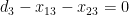
Notice, for every unit of flow sent along {(1,3)}, half a unit of flow must be sent along {(1,2)} and {(2,3)} as well to satisfy the cycle flow constraint.

The solution to this problem is {x_{13} = 600}, {x_{12} = -300}, {x_{23} = 900}, {s_1 = 300}, {s_2 = 1200} and {d_3 = 1500}. What is remarkable about this not all of customer 3’s demand is met by the lowest cost producer even though that producer has unlimited capacity. Why is this? The intuitive solution would have been send 600 units along {(1,3)} and 900 units along {(1,2) \rightarrow (2,3)}. This flow violates the cycle constraint.

In this example, when generator 1 injects electricity into the network to serve customer 3’s demand, a positive amount of that electricity must flow along every path from 1 to 3 in specific proportions. The same is true for generator 2. Thus, generator 1 is unable to supply all of customer 3’s demands. However, to accommodate generator 2, it must actually reduce its flow! Hence, customer 3 cannot contract with generators 1 and 2 independently to supply power. The shared infrastructure requires that they co-ordinate what they inject into the system. This need for coordination is the argument for a clearing house not just to manage the network but to match supply with demand. This is the argument for why electricity markets must be designed.

The externalities caused by electricity flows is not a proof that a clearing house is needed. After all, we know that if we price the externalities properly we should be able to implement the efficient outcome. Let us examine what prices might be needed by looking at the dual to the surplus maximization problem.

Let {y_i} be the dual variable associated with the flow balance constraint. Let {\lambda_C} be associated with the cycle constraints. Let {\nu_i} and {\theta_i} be associated with link capacity constraints. Let {\mu_i} and {\sigma_i} be associated with the remaining tow constraints. These can be interpreted as the profit of supplier {i} and the surplus of customer {i} respectively. For completeness the dual would be:

\displaystyle \min \sum_{(i,j) \in E}[\nu_{ij} + \theta_{ij}]K_{ij} + \sum_{i \in V}[S_i \mu_i + D_i \sigma_i]

subject to

\displaystyle -\theta_{ij} + \nu_{ij} + \rho_{ij}\sum_{C^+ \ni (i,j)}\lambda_C - \rho_{ij}\sum_{C^- \ni (i,j)}\lambda_C + y_i - y_j = 0\,\, \forall (i,j) \in E

\displaystyle \mu_i - y_i \geq -c_i\,\, \forall i \in V

\displaystyle \sigma_i + y_i \geq v_i\,\, \forall i \in V

\displaystyle \nu_{ij}, \theta_{ij}, \mu_i, \sigma_i \geq 0\,\, \forall i \in V,\,\,\forall (i,j) \in E

Now {y_i} has a natural interpretation as a price to be paid for consumption at node {i} for supply injected at node {i}. {\mu_i} and {\nu_i} can be interpreted as the price of capacity. However, {\lambda_C} is trickier, price for flow around a cycle? It would seem that one would have to assign ownership of each link as well as ownership of cycles in order to have a market to generate these prices.