A Lovely Proof (?) of Minimax

Peter Bickel taught me a nifty, little, literally, proof of the minimax theorem. Peter says it was inspired by his reading of David Blackwell‘s vector generalization of the same. Here goes.

Let be the payoff matrix of zero-sum game. Here is the payoff to the row player from playing when the column player plays . Let be $k$-simplex.

For each , let This is the set of payoffs that the row player can achieve when playing mixed strategy . By convexity, it must be an interval whose endpoints depend on . We will only be interested in the left most endpoint, call it . Thus, we can assume that (strictly speaking should be subset) Similarly, for each , let . By the same observations we may suppose that

For any and we have Now, choose which exists by continuity and compactness. Similarly, choose Then, is the value of the game.

No Farkas or separating hyperplane. Now, minimax is equivalent to duality. So, one might wonder whether such a proof could be used to obtain the duality theorem of linear programming. Assuming that the primal and the dual had optimal solutions, yes. However, the case where one is infeasible or unbounded would cause this kind of proof to break.

PS: Then, Olivier Gossner pointed out that perhaps because I wanted to believe so much that it was true, that I had overlooked something. See the comments. He was right. I tried to make the proof work but could not. A proof of minimax that avoids Farkas and/or the separating hyperlane is not outlandish. There is Guillermo Owen’s proof, via induction, for example. By the way this was not the first such elementary proof. There was a flurry elementary proofs of the minimax in the 40s and 50s in response to a challenge of von Neumann. Indeed, Peck (1958) writes in the introduction to his paper:

“There are so many proofs of this theorem in the literature, that an excuse is necessary before exhibiting another. Such may be found by examining the proof given below for the following: it uses no matrices, almost no topology and makes little use of the geometry of convex sets; it applies equally well to the case where only one of the pure strategy spaces is finite; also there is no assumption that the payoff function is bounded.”

That an induction proof should exist is unsurprising given David Gale’s inductive proof of the Farkas lemma. In fact, Gale’s proof can be seen as an instantiation of Fourier’s method for solving linear programs, again, no Farkas or separating hyperplane.

Lloyd Shapley

I am not the right person to write about Lloyd Shapley. I think I only saw him once, in the first stony brook conference I attended. He reminded me of Doc Brown from Back to The Future, but I am not really sure why. Here are links to posts in The Economist and NYT following his death.

 

Shapley got the Nobel in 2012 and according to Robert Aumann deserved to get it right with Nash. Shapley himself however was not completely on board: “I consider myself a mathematician and the award is for economics. I never, never in my life took a course in economics.” If you are wondering what he means by “a mathematician” read the following quote, from the last paragraph of his stable matching paper with David Gale

The argument is carried out not in mathematical symbols but in ordinary English; there are no obscure or technical terms. Knowledge of calculus is not presupposed. In fact, one hardly needs to know how to count. Yet any mathematician will immediately recognize the argument as mathematical…

What, then, to raise the old question once more, is mathematics? The answer, it appears, is that any argument which is carried out with sufficient precision is mathematical

 

In the paper Gale and Shapley considered a problem of matching (or assignment as they called it) of applicants to colleges, where each applicant has his own preference over colleges and each college has its preference over applicants. Moreover, each college has a quota. Here is the definition of stability, taken from the original paper

Definition: An assignment of applicants to colleges will be called unstable if there are two applicants and who are assigned to colleges and , respectively, although prefers to and prefers to .
According to the Gale-Shapley algorithm, applicants apply to colleges sequentially following their preferences. A college with quota maintains a `waiting list’ of size with the top applicants that has applied to it so far, and rejects all other applicants. When an applicant is rejected from a college he applies to his next favorite college. Gale and Shapley proved that the algorithm terminates with a stable assignment.

One reason that the paper was so successful is that the Gale Shapley method is actually used in practice. (A famous example is the national resident program that assigns budding physicians to hospitals). From theoretical perspective my favorite follow-up  is a paper of Dubins and Freedman “Machiavelli and the Gale-Shapley Algorithm” (1981): Suppose that some applicant, Machiavelli, decides to `cheat’ and apply to colleges in different order than his true ranking. Can Machiavelli improves his position in the assignment produced by the algorithm ? Dubins and Freedman prove that the answer to this question is no.

Shapley’s contribution to game theory is too vast to mention in a single post. Since I mainly want to say something about his mathematics let me mention Shapley-Folkman-Starr Lemma, a kind of discrete analogue of Lyapunov’s theorem on the range of non-atomic vector measures, and KKMS Lemma which I still don’t understand its meaning but it has something to do with fixed points and Yaron and I have used it in our paper about rental harmony.

I am going to talk in more details about stochasic games, introduced by Shapley in 1953, since this area has been flourishing recently with some really big developments. A (two-player, zero-sum) stochastic game is given by a finite set of states, finite set of actions for the players, a period payoff function , a distribution over for every state and actions , and a discount factor . At every period the system is at some state , players choose  actions simultaneously and independently. Then the column player pays to the row player. The game then moves to a new state in the next period, randomized according to . Players evaluate their infinite stream of payoofs via the discount factor . The model is a generalization of the single player dynamic programming model which was studied by Blackwell and Bellman. Shapley proved that every zero-sum stochastic game admits a value, by imitating the familiar single player argument, which have been the joy and pride of macroeconomists ever since Lucas asset pricing model (think Bellman Equation and the contraction operators). Fink later proved using similar ideas that non-zero sum discounted stochastic games admit perfect markov equilibria.

A major question, following a similar question in the single player setup, is the limit behavior of the value and the optimal strategies when players become more patient (i.e., goes to ). Mertens and Neyman have proved that the limit exists, and moreover that for every there strategies which are -optimal for sufficiently large discount factor. Whether a similar result holds for Nash equilibrium in -player stochastic games is probably the most important open question in game theory. Another important question is whether the limit of the value exists for zero-sum games in which the state is not observed by both players. Bruno Zilloto has recently answered this question by providing a counter-example. I should probably warn that you need to know how to count and also some calculus to follow up this literature. Bruno Zilloto will give the Shapley Lecture in Games2016 in Maastricht. Congrats, Bruno ! and thanks to Shapley for leaving us with some much stuff to play with !

Who Was Colonel Blotto?

Credit for the game that bears his name is due to to Borel. It appears in a 1921 paper in French. An English translation (by Leonard Savage) may be found in a 1953 Econometrica.

 

The first appearance in print of a version of the game with Colonel Blotto’s name attached is, I believe, in the The Weekend Puzzle Book by Caliban (June 1924). Caliban was the pen name of Hubert Phillips one time head of Economics at the University of Bristol and a puzzle contributor to The New Statesman.

Blotto itself is a slang word for inebriation. It does not, apparently, derive from the word `blot’, meaning to absorb liquid. One account credits a French manufacturer of delivery tricycles (Blotto Freres, see the picture) that were infamous for their instability. This inspired Laurel and Hardy to title one of their movies Blotto. In it they get blotto on cold tea, thinking it whiskey.

Over time, the Colonel has been promoted. In 2006 to General and to Field Marshall in 2011.

Expert testing part 3

Department of self-promotion: sequential tests, Blackwell games and the axiom of determinacy.

Links to part 1 and part 2

Recap: At every day an outcome is realized (`‘ means a rainy day, `‘ a non-rainy day). An expert claims to know the distribution of the stochastic process that generates the sequence of outcomes. A sequential test is given by a Borel set of infinite sequences of predictions and outcomes. An expert who delivers forecast fails on a realization if where is the prediction made by about given the previous outcomes .

Let me remind you what I mean by `a test that does not reject the truth with probability ‘. I am going to write an equivalent definition to the one I used up to now, this time using the language of stochastic processes.

Definition 1 The test does not reject the truth with probabality if for every -valued stochastic process one has

where

We are going to prove the following theorem:

Theorem 2 Consider a sequential test that does not reject the true expert with probability . Then for every there exists a such that

for every .

So a charlatan, who doesn’t know anything about the true distribution of the process, can randomize a forecast according to and pass the test with high probability regardless of the actual distribution.

— Discussion —

Before we delve into the proof of the theorem, a couple of words about where we are. Recall that a forecast specifies the Expert’s prediction about rain tomorrow after every possible history . We denote by the set of all such forecasts. The most general tests are given by a function , and specify for every such the set of realizations over which the forecast fails. Since is infinite we know that there exist tests that passes a true expert and are not manipulable by a strategic charlatan.

Sequential tests have the additional property that the test’s verdict depends only on predictions made by along the realized path: When deciding whether a forecast passes or fails when the realization is the test only considers the predictions made by along x. We also say that the test does not depend on counter-factual predictions, i.e. predictions about the probability of rainy day after histories that never happen. It seems that counter-factual predictions would be irrelevant to testing anyway, but, as the theorem shows, if the test does not use counter-factual prediction then it is manipulable.

One situation in which sequential tests are the only available tests is when, instead of providing his entire forecast before any outcome is realized, at every day the expert only provides his prediction about the outcome of day just before it is realized. At infinity, all the information available to the tester is the sequence of predictions and realized outcomes.

— Sketch of Proof —

We can transform the expert’s story to a two-player normal form zero-sum game as we did before: Nature chooses a realization and Expert chooses a forecast . Then Expert pays Nature if fails on and otherwise. The fact that the test does not reject the true expert translates to the fact that the maximin of the game is small. If we knew that the minimax is also small then an optimal mixed strategy for the Expert will satisfy (3). We only need to prove the existence of value, or as game theorists say, that the game is determined.

Unfortunately, this time we cannot use Fan’s Theorem since we made no topological assumption about the set , so there is no hope to get semi-continuity of the payoff function. Indeed, as we shall see in a moment, the Normal form representation misses an important part of the expert’s story. Instead of using a normal form game, we are going to write the game in extensive form. I will call this game .

1. The game is played in stages .
2. At stage Nature chooses an outcome and Expert chooses a prediction simultaneously and independently.
3. Nature does not monitor past actions of Expert.
4. Expert monitors past actions of Nature.
5. At infinity, Expert pays Nature if and otherwise.

Now I am going to assume that you are familiar with the concept of strategy in extensive form game, and are aware of Kuhn’s Theorem about the equivalence between behavioral strategies and mixtures of pure strategies (I will make implicit uses of both directions of Kuhn’s Theorem in what follows). We can then look at the normal form representation of this game, in which the players choose pure strategies. A moment’s thought will convince you that this is exactly the game from the previous paragraph: Nature’s set of pure strategies is , Expert’s set of pure strategies is and the payoff for a strategy profile is . So far no real gain. Extensive form games in which one of the players don’t monitor opponent’s actions need not be determined. In order to get a game with a value we are going to twist the game , and allow Nature to observe past actions of the Expert player. This makes life more difficult for the Expert. Up to a minor inaccuracy which I will comment about later, the resulting game is what’s called Blackwell game and it admits a value by (a seminal theorem of Donald Martin).

Here is the game after the twist. I call this game .

1. The game is played in stages .
2. At stage Nature chooses an outcome and Expert chooses a prediction simultaneously and independently.
3. Each player monitors past actions of the opponent.
4. At infinity, Expert pays Nature if and otherwise.

Now if you internalized the method of proving manipulability that I was advocating in the previous two episodes, you know what’s left to prove: that the maximin of is small, i.e. that, fore every strategy of Nature, Expert has a response that makes the payoff at most . We know this is true for the game but in Nature is more powerful.

Here is the most important insight of the proof: The fact that an expert who knows the distribution of the process can somehow pass the test implies that the maximin in is small, but this fact alone doesn’t say anything about the maximin of . To show that the maximin of is also small we will use the fact that the way such an expert passes the test is by providing the correct forecast. Until now the distinction was not really important to us. Now it comes into play.

Let be a behavioral strategy of Nature in , i.e. a contingent plan that specifies the probability that Nature play after every. Let be the pure strategy of Expert in that is given by

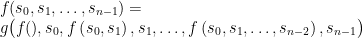
So the pure action taken by the Expert player at day is the mixed action that Nature is going to take at day according to her strategy . Now assume that Nature follows and Expert follows . Let and be the random variables representing the actions taken by Expert and Nature at day . Then the stochastic process satisfies (2). Therefore from (1) we get that the expected payoff when Nature plays and Expert plays is indeed smaller than .

Now for the minor inaccuracy that I mentioned: For Martin’s Theorem we need the set of actions at every stage to be finite. We can handle this obstacle by restricting Expert’s action at every stage to a grid and applying the coupling argument.

— Non-Borel Tests —

What about pathological sequential tests that are given by a non-Borel set ? Well, if, like me, you find it preposterously impossible to choose one sock from each of infinitely many pairs of socks, then perhaps you live in the AD paradise. Here every set is measurable, Blackwell Games are determined even when the payoff function is not Borel, and Theorem 2 is true without the assumption that is Borel. See, the AD universe is a paradise for charlatans, since they can do as well as the true experts.

If, on the other hand, you subscribe to the axiom of choice, then you have a non-manipulable test:

Theorem 3 There exists a sequential test with a non-Borel set that does not reject the truth with probability and such that for every there exists some realization such that

— Summary —

If you plan to remember one conclusion from my last three posts, I suggest you pick this: There exist non-manipulable tests, but they must rely on counter-factual predictions, or be extremely pathological.

Muchas gracias to everyone who read to this point. Did I mention that I have a paper about this stuff ?

Lecture notes on expert testing

I am visiting the rationality center in the Hebrew University, and I am presenting some papers from the expert testing literature. Here are the lecture notes for the first talk. If you read this and find typos please let me know. The next paragraph contains the background story, and can be safely skipped.

A self-proclaimed expert opens a shop with a sign at the door that says `Here you can buy probabilities’. So the expert is a kind of a fortune-teller, he provides a service, or a product, and the product that the expert provides is a real number: the probability of some event or more generally the distribution of some random variable. You can ask for the probability of rain tomorrow, give the expert some green papers with a picture of George Washington and receive in return a paper with a real number between 0 and 1. The testing literature asks whether you can, after the fact, check the quality of the product you got from the expert, i.e. whether the expert gave you the correct probability or whether he just emptied your pocket for a worthless number.

So, let be a set of realizations. Nature randomizes an element from according to some distribution and an expert claims to know Nature’s distribution. A test is given by a function : the expert delivers a forecast and fails if the realization turned out to be in . A good test will be such that only `true’ experts, i.e. those who deliver the correct , will not fail.

— Manipulability —

I start with Sandroni’s paper (pdf). The following definition formalises the idea that the true expert is unlikely to fail the test

Definition 1 The test does not reject the truth with probability if for every .

If a test does not reject the truth with probability then a true expert, who knows how nature randomizes the realization, is unlikely to fail the test. Alas, a charlatan who acts strategically is also unlikely to fail

Theorem 2 (Sandroni (2003)) Let be finite. If is a test that does not reject the true expert with probability then there exists such that for every .

So, a charlatan who knows nothing about how Nature chooses can randomize a forecast according to , and is unlikely to fail, regardless of the realization. We say that the test is manipulable.

For Sandroni’s Theorem we do not need to assume any structure on . However the situation we have in mind is that for some finite set of outcome. So at every day Nature randomizes an outcome of and the Expert claims to know the stochastic process that governs Nature’s choices.

Proof: Let be a finite set such that .

Consider the following two-player zero-sum game with the players called Nature and Expert. Nature is the maximizer with pure strategies set , and Expert is the minimizer, with pure strategies set . If Nature plays and Expert plays then Expert pays Nature if and otherwise.

By von-Neumann’s Minimax Theorem the game admits a value in mixed strategies, so that the maximin equals the minimax. We claim that . Indeed, let be a mixed strategy of Nature and let be such that . Then the expected payoff that Expert pays Nature if Nature plays and Expert plays is since the game does not reject the true expert with probability .

Now let be a mixed optimal strategy of the Expert in the game. Then

for every pure strategy of Nature, since the left hand side is the expected payoff that the Expert pays Nature if he plays and Nature plays .

The argument in the proof of Sandroni’s Theorem captures the essence of all the manipulability theorems we will see. We define a zero-sum game between two players, Nature and Expert. The minimax theorem is the core of the proof: The fact that the maximin is smaller than follows from the assumption that the test is unlikely to reject the true expert. The fact that minimax is smaller than implies that the test is manipulable. In the middle, we use the most wonderful miracle that the minimax and maximin are equal.

— Fan’s Theorem —

Here is the more general minimax theorem which we will use later: In a zero-sum game, if one of the players have a compact set of pure strategies, and the payoff to that player is u.s.c. in his own strategy then the game admits a value in mixed strategies.

Proposition 3 (Ky Fan)Consider a two-player zero-sum game in normal form with pure strategy sets and payoff function . If is a compact metrizable space and is upper-semi continuous for every then the game has a value in mixed strategies, i.e.

and all suprema are attained.

The set is not topologized and is the set of distributions over with finite support, so the integral on the right side is just a summation. The challenge in using Fan’s Theorem is to find a topology over which is sufficiently weak to make compact and sufficiently strong to make the functions upper semi-continuous.

— Non-manipulability —

Sandroni’s Theorem does not hold when is infinite, precisely because the game we defined in the proof will have no value. We now take a game without a value and translate it to a non-manipulable test for an infinite set of realizations. I only know about one game without a value (`I know a larger such game’ quipped Sergiu when I said it in the talk): Two players pick simultaneously and independently natural numbers and the player that chose the largest number wins. Here is the translation of the game to a test:

Example 1 Let . Let be the test that is given by

Then does not reject the true expert with probability , and for every there exists a realization such that

Not only the test is not manipulable, also for every that a charlatan might employs to randomize his worthless forecast , there is some realization under which he fails with high probability.

Proof: For every let ( for tail) be given by . Then can be equivalently written as .

We first show that the test has small probability to reject a true expert. Indeed,

for every , where the first equality follows from the definition of and the second from the definition of .

Now let . Let be the push-forward of under and let . Then

The first equality follows from the definition of , the second from the definition of and the inequality from the choice of .

— Sequential Tests —

So, Sandroni’s Theorem only holds for finite sets . We are now aiming at proving a manipulability theorem for infinite set by adding some structure on the set and some restrictions on the test. From now on we assume that . The set is the set of outcomes. Everything works for arbitrary finite set of outcomes but I stick with two outcomes for notational convenience. Note that a compact metrizable space in the product topology.

There is an almost equivalent representation of and element as the conditional probability that given for a -randomly chosen . Let be the set of functions , then this gives rise to natural map , which is surjective and continuous when the domain is equipped with the product topology and the range with the weak topology. It will be useful to identify with , so I will think of a test as a function .

For every and every realization , the sequence of forecasts of along is given by where .

Definition 4 A test is sequential if implies for every and every realization such that the forecasts made by and along are the same.

Equivalently, a sequential test is given by a subset ( for rejection): iff for every realization and every forecast , where is the sequence of predictions of along .

— Next Episode (Thursday 12:00) —

I will talk about Olszewski and Sandroni’s paper `The manipulability of future independent tests’ and my paper `Many inspections are manipulable’ . Main goal is to prove that sequential tests are always manipulable.

A post on Rabin

I wrote some time ago about Michael Rabin’s example of how a backward induction argument is killed when you require players’ plans to be computable. Since Rabin’s paper is not available online, I intended to post the proof at some point, but never actually got to do it. Richard Lipton’s post about Emil Post is a good inspiration to pay that debt since the concept of simple set, which was introduced by Post, has a role in Rabin’s example.

A set is simple if is recursively enumerable and its complement is infinite and contains no infinite recursively enumerable subset.

For Rabin’s purpose, what matters is that Post proved the existence of such a set. So Post provides us with a code of a computer program that enumerates over all the elements of and such that no computer program can produce infinitely many elements that are not in . By the way, Post introduces the concept of simple set while working on his eponymous problem which Richard mentions. In fact, if is simple set then is not many-one equivalent to a universal recursively enumerable set.

Now let be a simple set and consider the following three-round game with perfect information. At each round a player announces a natural number (an action): First Alice announces . Then Bob announces and then Alice announces . After the game is played, a winner is determined as follows: Bob wins if and is not the -th element in the enumeration of . Otherwise, Alice wins. Therefore, determining the winner is a task that can be effectively done using the code provided by Post.

Does any of the players have a strategy that guarantee winning regardless of how the opponent play ? The answer to this question depends on which mathematical creature you use to model the intuitive notion of `strategy’.

If by a strategy you mean just a function from histories to current action then Bob has a winning strategy: for every that Alice might chose in the first round there exists some such that , since the complement of is infinite.

But if you think of a strategy as a complete set of instructions, that is a plan or an algorithm that will tell you how to produce your next action given the past, then you want to model a strategy as a computable function. Now, for every computable function that Bob can chose, there exists some such that either or since otherwise would have been a recursive enumeration of infinitely many elements of . In particular, there exists some such that if Alice plays in the first stage and in the third stage she wins against . So, Bob has no winning strategy.

Computability in game theory

Since in the near future I will have to start advocating a computability argument, and since this position is somewhat in contrast to what was my view a couple of years ago when I first came across algorithmic game theory, I thought I should try to clarify my thoughts about the issue in a couple of posts.

The most beautiful example I know for the surprising outcomes we get when taking computability into account in game theory is Michael Rabin’s paper from 1957. Rabin considers a finite win-loss game with perfect information between two players, Alice and Bob. The game is played in three rounds, at each round a player announces a natural number (an action): First Alice announces . Then Bob announces and then Alice announces . After these declaration are made, the game coordinator determines the winner: If Alice wins. If Bob wins. The set , Alice’s winning set, is part of the description of the games. This is a finite game, which can be solved by a background induction. By the so called Zermelo’s Theorem, the game is determined: One of the player has a winning strategy. The identity of the winner depends of course on .

Rabin gives an example for a game with the following propertie:

1. is a decidable set: this means that there is an effective way to decide, for every triple whether or not . So the job of the game coordinator in this game can be performed by a computer program. Games with effectively computable payoff are called actual games: These are the games that can actually be played.
2. Bob has a winning strategy : whatever actions and Alice chooses in the first and third stages, Bob will win the game if in the second stage he chooses : so that for any
3. Bob has no computable winning strategy: For every function that can be computed by a computer program there exist some actions for Alice such that .

Feel the blow ? Bob finds himself in a strange predicament. On the one hand, after observing Alice’s action from the first round, Bob knows that there is some action he can choose that beats any possible response of Alice. However, if Bob tries to `plan ahead’ which action to take after every possible choice of , he cannot produce such a plan. Bob can beat all Alice’s strategies and Alice can beat all Bob’s (computable) strategies. von-Neumann and Morgenstern’s least controversial idea, solving a zero-sum game with perfect information by backward induction, trembles. The argument that in finite zero-sum games with perfect information a player doesn’t care if the opponent finds out his strategy falls apart.

(To be continued…)